The Hitchhiker's Guide to Sizing

A robust framework for transforming risk from an arbitrary input into a controlled portfolio output

This guide is inspired by the risk management system introduced by Robert Carver in his book Systematic Trading. Despite its name, the book is also an excellent read for discretionary traders looking for systematic sizing.

Sizing a trade is often either oversimplified or overcomplicated. You will frequently hear that risking 1% per trade is a good rule of thumb, but is it really? Other investors sit at the opposite end of the spectrum, finding comfort in highly complicated models that run large covariance matrices with backward looking optimisation, only to realise that during market crises, correlations become unstable and often shift to 100%. Risk management that is too simple leads to erratic day-to-day volatility in your portfolio. Conversely, a system that is too complicated gives the illusion of perfect control over risks when, in fact, you do not have it.

“Uncertainty is an uncomfortable position. But certainty is an absurd one.” — Voltaire

At the end of the day, managing risk in a portfolio comes down to answering one question: How much risk do you want to take, and how confident are you? So let’s start with the latter: confidence.

Forecasting

When entering a trade, you should assign a level of confidence to it. For example, you might be very bullish on a stock, or simply bullish. This represents your forecast for the asset’s performance—a discretionary input to your risk management system, with values ranging from -20 to +20.

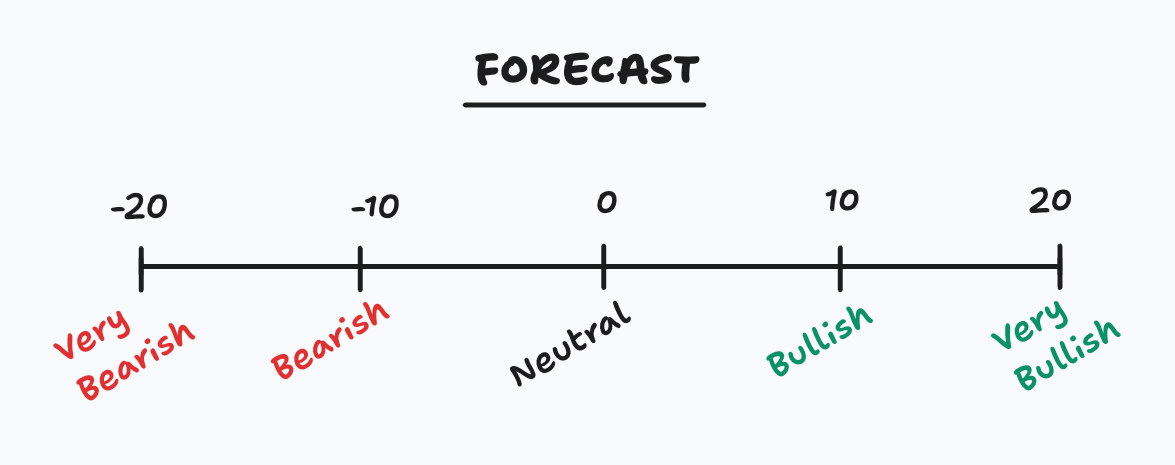
The Golden Rule of Forecasting: Over time, your average absolute forecast must be 10. This means most trades are a standard +/-10.

Reserve a +/-20 forecast for "Perfect Storm" setups where technical, fundamental, and macroeconomic factors all align.

If you are new or lack a tangible track record, stick strictly to +/-10. Scaling down to +/-5 is also a valid way to test new signals without over-committing capital.

Volatility targeting

The most important input to your risk management system comes from answering the question: How much risk do you want to take? This is not an easy question to answer—after all, what is risk, and how do you even measure it? We will keep it simple for now: risk is best measured by the expected standard deviation of the portfolio’s returns, also known as its volatility.

Let’s assume you are running a portfolio of $1 million. After spending some time on WallStreetBets, you decide that your target volatility is 69%. Truly a great number for outperforming your neighbours by trading meme stocks. But can you cope with that volatility?

To put things in perspective, because volatility scales with the square root of time, 69% annual volatility means that on average your portfolio will move by +/-4.31% per day (69% / √252). You should expect that 3.33 days in a month your portfolio will be down by more than -4.31%, and 5 days a year it will be down by more than -8.62%.

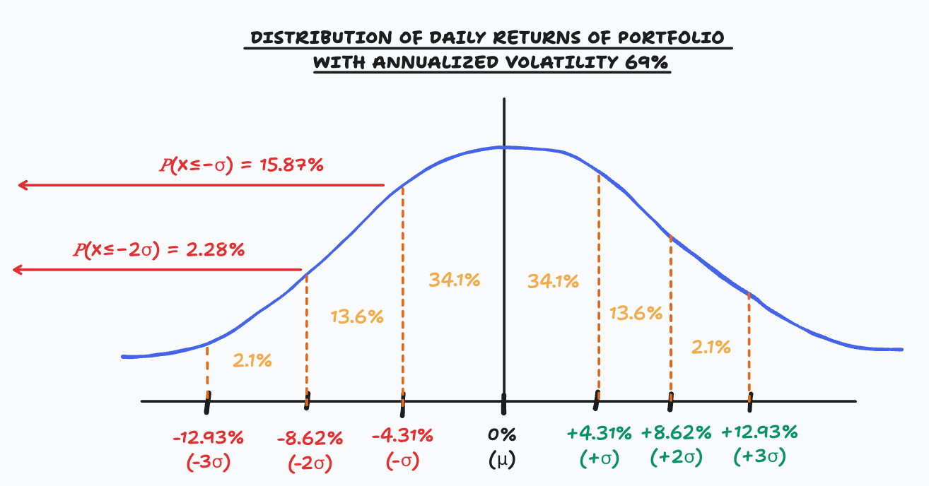
I’m not sure about you, but personally, I can’t cope with that level of daily volatility in my portfolio. NGMI, right…

And the above figures are just based on daily normal uncorrelated returns. Introduce some autocorrelation between the returns—or what we call strong momentum—and you see where this can go: either a glorious run for the portfolio or a catastrophic rout sending it into a very deep drawdown. Big drawdowns are what kill returns: after losing 50%, you need a 100% return to break even. Good luck with that.

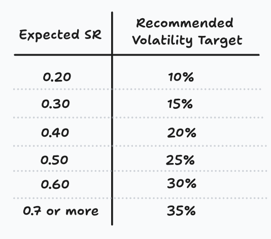
While everyone has a different risk appetite, we can still infer a recommended range of volatility targets. The only thing you need is your expected Sharpe Ratio (SR). Knowing your SR is no small feat, however—even with a solid backtest over many years, the SR remains a random variable following an unknown distribution. It can be positive on average, but inevitably some years will be negative. So I urge you to be conservative when selecting your expected Sharpe Ratio. Anything above 0.70 is too optimistic; yes, you can achieve a Sharpe >1.0 for years, but you are not immune to volatility, mean reversion, or the gravitational pull of a drawdown.

Below are the recommended volatility targets based on a half-Kelly criterion. While the full Kelly criterion identifies the mathematically optimal bet size to maximise long-term growth, it is notoriously aggressive and sensitive to errors in your assumptions. By using half-Kelly, we create a heuristic safety buffer that protects the portfolio against over-leveraging and the inevitability of a drawdown.

Note: If you are running a strategy with negative skew, such as harvesting equity volatility premium by selling options, you should divide the recommended volatility target by 2. Any volatility measured in a short convexity strategy is always underestimated. Don’t be stupid (looking at you, theta gang).

X-factor: average holding period

Traditionally, trading systems use simple money management: they allocate a certain percentage of trading capital to risk on each trade. The natural question, then, is how to link this capital at risk with volatility targeting at the portfolio level.

Consider Trader A, who risks 1% of his account on a daily intraday strategy. To simplify, assume one trade per day, a 50% win rate, and a 1:1 risk/reward ratio. On average, this trader risks 1% to make 1%. What is the annualized volatility of his portfolio? The answer is 15.87%. Volatility scales with the square root of time, so 1% daily volatility multiplied by the square root of 252 trading days yields 15.87%.

Now consider Trader B, who also risks 1% of his account but on a monthly swing trading strategy. Using the formula, the annualized portfolio volatility is 3.46% (1% × √12). As you can see, the expected portfolio volatility is much lower despite risking the same percentage per trade.

There is a direct relationship between the capital at risk per trade and the expected holding period of each trade. To achieve a desired annual target volatility at the portfolio level, you must account for the frequency and expected holding time of your strategy when determining the capital at risk per trade. In other words—contrary to common belief—the capital at risk per trade is not an input but an output of the risk management system.

You might now wonder how to know the expected holding time of a trade in advance. In the simple case of a buy-and-hold position, the trade remains open as long as technically possible. If you buy a stock on a cash account without margin, you can hold it indefinitely or until a corporate event occurs. At the opposite extreme, buying with leverage and a tight stop loss means the trade will likely last only a short time. The expected life of a trade depends directly on the distance to the stop loss.

From now on, I will assume we trade every position with a trailing stop loss. This creates trades with positive skew and a finite expected life. To scale the stop loss independently of the instrument’s volatility, we measure the distance to the stop loss in daily standard deviations—this is known as the X-factor.

Example:

1. SPY: Let’s assume the realized volatility on this ETF is 16%. The daily standard deviation is therefore 1% (16% / √252). If I place my stop loss 1% below my entry, that means I used an X-factor of 1. If I place it 3% below, the X-factor is 3, and so on.

2. NVDA: Volatility is 40%, so the daily standard deviation is 2.5%. A stop loss with an X-factor of 3 means the stop loss is 7.5% below my entry.

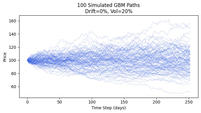
Unfortunately, when using a trailing stop loss, I don’t know of any straightforward mathematical formula to calculate the expected holding period based on the normalized distance to the stop loss. But fortunately, Monte Carlo simulations are perfect for this!

We can use geometric Brownian motion to simulate theoretical asset price paths. Below is an example of 100 simulated paths:

I ran a script with 50,000 simulated paths, and for different X-factor levels (1, 2, 3, 4, 6, and 8), I plotted the distribution of the holding periods. Using a trailing stop loss yields a log-normal distribution, which is to be expected: many trades get stopped out quite early, while a few winners remain open for long periods. This also illustrates the benefit of using a stop loss: it removes the left-tail risk of holding onto losers and lets winners run.

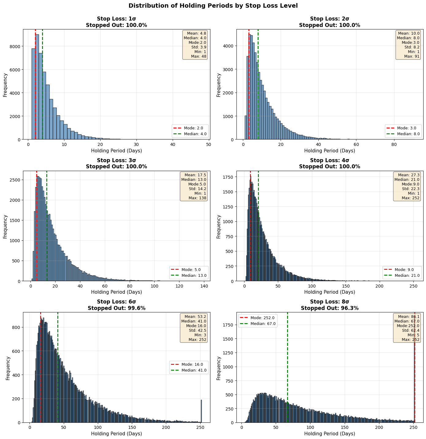
From the chart above, we can map an expected holding period to each X-factor stop loss level:

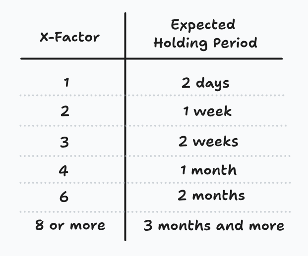
This table is a good rule of thumb but it should be taken with a grain of salt. First, the Monte Carlo simulations were generated with zero drift and constant volatility, which is a strong assumption. Second, the distribution of holding periods is log-normal, so the expected holding period falls roughly between the mode and the median of the distribution. When trading such a system, it might feel painful and uncomfortable because mode < median < mean: the most likely outcome is to get stopped out in a short period, while the average holding period is stretched much further due to outliers. The mental pain of getting stopped out is the price to pay for outsized returns in the long run.

Sizing one bet at a time

Now that we have defined volatility targeting, forecasts, and the X-factor, we can finally examine how to size a trade in practice.

Consider a swing trader on S&P 500 futures; let’s call him John. This trader exclusively trades the same asset and never holds more than one position at a time in his portfolio.

After backtesting his strategy—or simply running it with low capital—John decides to scale up and follow our risk management system. Historically, his strategy has averaged a Sharpe ratio of 0.90, but John is conservative, so he assumes he can deliver at least 0.6. According to the table introduced earlier, this leads him to a volatility target of 30%. Running the strategy on a $1 million trading account, he expects daily P&L volatility of +/- $18,750. He considers that an acceptable dollar amount given his risk appetite.

On average, John trades in and out of S&P 500 futures every week; that is his expected holding period. According to the X-factor table from the previous section, John should use an X-factor of 2.

John currently has no open position, but this morning he receives a buy signal. The signal is neither weak nor strong; he has average confidence in it, so his forecast for the trade is +10.

John checks the annualized realized volatility of S&P 500 returns over the last month and finds 14.50%.

Now John has all the inputs needed to compute the trade size:

\(\begin{align*} \text{Instrument Notional} &= \frac{\text{Forecast}}{10} \times \frac{\text{Target Volatility}}{\text{Instrument Volatility}} \times \text{Account Value} \\ &= \frac{10}{10} \times \frac{30\%}{14.50\%} \times \$1,000,000 \\ &= \$2,068,965 \end{align*}\)

He needs to buy $2,068,965 worth of S&P 500 futures, effectively introducing leverage of 206.97% into his $1 million trading account.

The stop loss calculation is straightforward:

\(\begin{align*} \text{Instrument Stop Loss} &= \frac{\text{Instrument Volatility}}{\sqrt{252}} \times \text{X-factor} \\ &= \frac{\text{14.5%}}{\sqrt{252}} \times 2 \\ &= \text{1.82%} \\ \end{align*}\)

John will need to place a stop loss 1.82% below his entry price.

At the account level, this 1.82% instrument stop loss means John is risking 1.82% × 206.97% = 3.77% of his capital, or $37,700. This might seem large, but it is the amount he must put at risk to achieve his 30% annual portfolio volatility target. No pain no gain!

There is a handy simple approximation formula to double-check our calculation. Assuming John risks 3.77% every week, we can compute the expected annualized volatility for this trading account as follows:

\(\begin{align*} \text{Expected Volatility} &\approx \text{Capital At Risk per trade} \times \sqrt{\text{Number of trades per year}} \\ &\approx \text{3.77%} \times \sqrt{52} \\ &\approx \text{27.19%} \\ \end{align*}\)

27.19% is close enough from our 30% volatility target.

This sizing system may feel counterintuitive at first, as traditional approaches treat capital at risk per trade as a fixed input. Here, however, it emerges as an output derived from three key elements: your desired annual portfolio volatility, the confidence level (forecast) in each trade, and the normalized stop-loss distance (X-factor) tied to expected holding periods.

This method is superior because it forces you to confront the central question of how much risk you truly want to bear over the full year before placing any trade. By aligning position sizes with your long-term risk appetite rather than arbitrary per-trade rules, it delivers a more resilient, consistent, and psychologically sustainable approach to risk management.

This is not a "set and forget" system. If an asset’s volatility rises, its risk weight has increased. You must re-calculate and likely sell some exposure to maintain your target. It is best practice to re-calculate whenever there is a significant change in market regime or realized volatility.

So far, we have only addressed the case of a trader with one position at a time, which is not what most traders or investors do. In the next section, we will examine the sizing of multiple bets held simultaneously in a portfolio.

Diversification: optimal number of active bets

Realistically, most traders and investors hold multiple positions simultaneously across various instruments or asset classes.

Diversification offers significant benefits. As Harry Markowitz famously stated, “Diversification is the only free lunch in investing”. This holds true in general: adding uncorrelated bets reduces overall portfolio volatility compared to concentrating on a single position, which can improve the expected Sharpe ratio.

However, diversification is not foolproof. Warren Buffett has cautioned against excess: over-diversification can lead to diworsification. In his words, “Diversification is protection against ignorance. It makes little sense if you know what you are doing”. Including more bets introduces hidden risks. During market stress, correlations often spike, transforming apparently uncorrelated positions into one large correlated bet. By the time this becomes evident, it is usually too late, and the portfolio suffers a severe drawdown.

So, should we diversify or concentrate? Sorry, folks, we are going to need a little math here, nothing too advanced though.

To explore this question, let us examine the formula for the total variance of a portfolio:

\(V_p = \sum_{i=1}^N \sum_{j=1}^N w_i w_j \rho_{ij} \sigma_i \sigma_j\)

with:

\(\begin{flalign*} V_p: &\text{ Variance of the portfolio's returns} \\ N_p: &\text{ Number of assets in the portfolio} \\ w_i: &\text{ Weight of asset }i \text{ in the portfolio} \\ w_j: &\text{ Weight of asset }j \text{ in the portfolio} \\ \rho_{ij}: &\text{ The correlation coefficient between the returns of assets }i\text{ and }j \text{ in the portfolio} \\ \sigma_i: &\text{ The standard deviation of the returns of asset }i\\ \sigma_j: &\text{ The standard deviation of the returns of asset }j\\ \end{flalign*}\)

In our case, we use risk-adjusted bets: each bet contributes the same amount of risk to the portfolio. This leads to the following assumptions:

\(\begin{flalign*} \text{Equally Weighted Portfolio: } &w_i=w_j=\frac{1}{N} \\ \text{Fully Invested Portfolio: } &\sum_{i=1}^N w_i = 1\\ \text{Equal Risk Bets: } &\sigma_i = \sigma_j = \sigma\text{ for all }i, j\\ \end{flalign*}\)

Then we can simplify the portfolio variance formula to:

\(V_p = \frac{\sigma^2}{N}+\frac{2 \sigma^2}{N^2} \sum_{i < j} \rho_{ij}\)

Edit: on mobile, the LaTeX formula is missing a “+” sign, this should read as sigma^2/N + 2sigma^2/N^2*Sum{rho_i_j}

The first term, σ²/N, represents the “idiosyncratic” or diversifiable risk from individual assets, which becomes diluted as you add more assets. Variance scales linearly with the number of assets, while standard deviation (what we call portfolio volatility) scales with the square root. As you add more assets, the marginal diversification benefit decreases.

The second term incorporates the pairwise correlations (ρ between i and j) and reflects “systematic” or undiversifiable risk due to how assets move together.

The formula strikes a balance between isolation (low correlations spread risk) and synchronization (high correlations amplify it). As correlations rise, portfolio variance increases, causing the portfolio to behave more like a single asset exposed to broad market risks, typically macroeconomic or other systemic factors. If you did not intend to take those risks, you have effectively diworsified your portfolio. Conversely, low or negative correlations shrink the second term and can even make it negative if enough pairs are negatively correlated (similar to a hedge), thereby reducing overall portfolio risk and creating the possibility of undershooting your target volatility.

In an idealized world, you would hold only uncorrelated bets. If all correlations are zero, you achieve perfect diversification nirvana: risk drops with the square root of the number of positions. In reality, correlations are not fixed. Even traditionally “uncorrelated” assets like stocks and bonds can become highly correlated during events such as inflation spikes.

It is easy to underestimate correlation, especially across asset classes. Correlations are not normally distributed: most of the time they appear low, but in crises or regime shifts they can spike dramatically alongside volatility. This creates the potential for severe drawdowns that wipe out months of profits and undermine the careful risk management you have built.

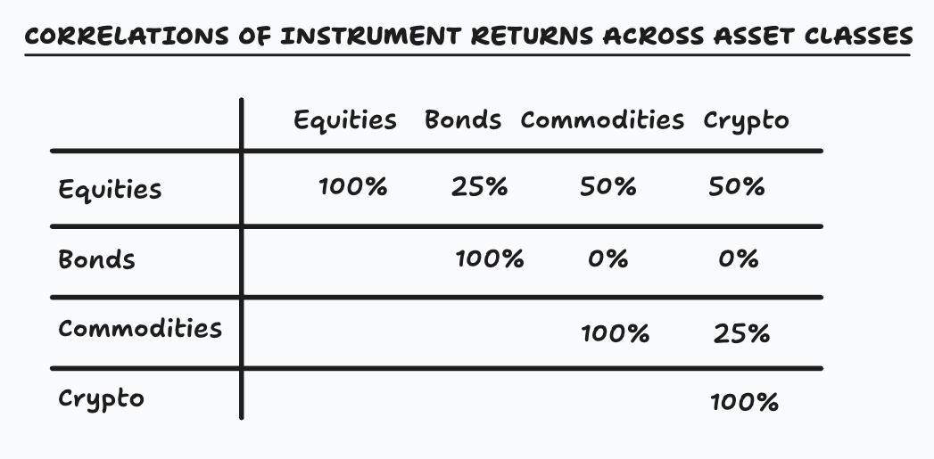
My solution is to avoid assuming correlation stability and to recognize that recent historical correlations are often poor predictors of future ones. Instead, I use conservative correlation assumptions and I aim for an average correlation target across my bets. The below table should be used as a rule of thumb for estimating correlation across bets using their instrument asset class. It doesn’t require any calculation and provide a good enough framework for achieving most of the diversification benefits.

If we assume an average pairwise correlation​, meaning that the correlations differ across pairs but we approximate their effect by using a single average value, the portfolio variance formula simplifies significantly into:

\(V_p = \frac{\sigma^2}{N} + \left(1 - \frac{1}{N}\right) \bar{\rho} \sigma^2\)

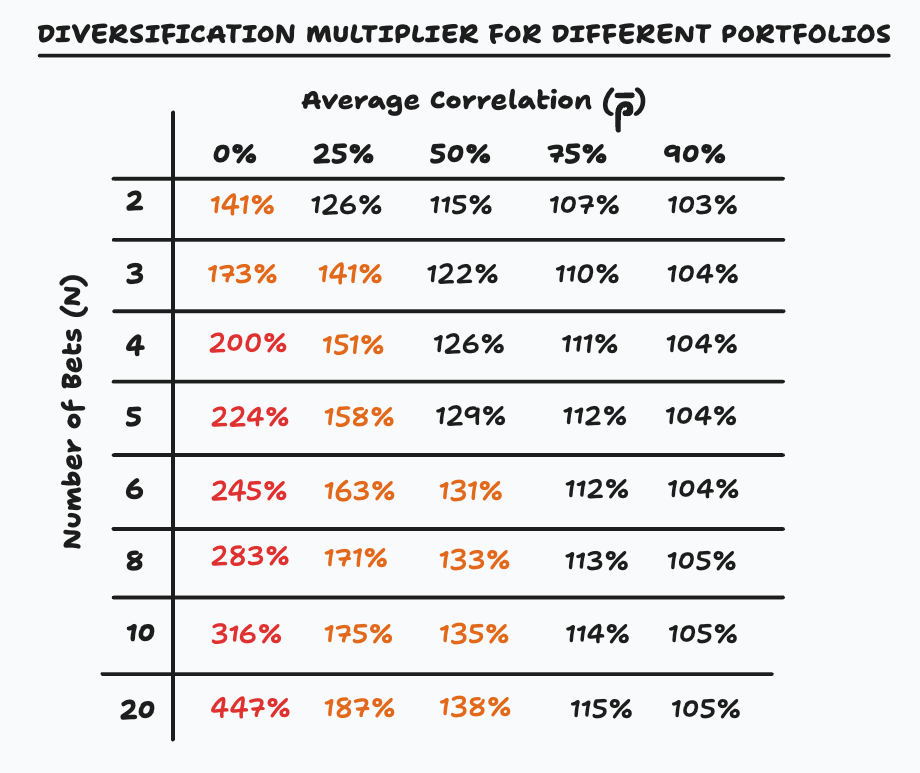
Using this formula, and assuming a volatility of 20% for each bets, we can easily compute the expected portfolio volatility for different level of average correlations and number of bets:

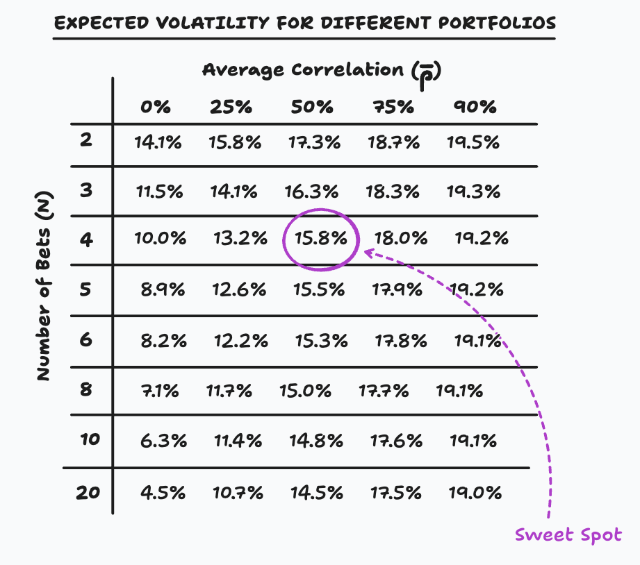
Unsurprisingly, adding more bets when correlation is high (90%) does not provide any benefits. It keeps the portfolio volatility very close to 20% and adds significant systematic risk—this is diworsification. However, adding more uncorrelated bets lower the overall portfolio volatility, and of course, the lower the correlation, the greater the diversification benefits. In reality, it is quite difficult to find many purely uncorrelated bets, and you will eventually stumble upon only 3 to 5 purely uncorrelated bets when trading or investing in traditional publicly listed assets. My sweet spot, and what I try to average over time, is to find 4 to 5 bets while aiming for an average correlation of 50%. This gives me enough diversification benefits while keeping the number of bets manageable. That’s my interpretation of Stanley Druckenmiller’s adage: “Put all your eggs in one basket and then watch that basket very carefully.”

Diversification multiplier

As we have seen in the previous section, adding low-correlated bets lowers the total portfolio variance. While this is excellent for achieving higher Sharpe ratios, it also means we are undershooting our volatility target. To address this issue, we need to increase the notional exposure of all our bets. This adjustment is known as the diversification multiplier. The multiplier is calculated by dividing the volatility target by the expected volatility of the portfolio. Using the previous table, we can compute the diversification multiplier for each pair of number of bets and average correlation.

We can now revisit the formula for computing the instrument notional for a given bet by incorporating the diversification multiplier.

\(\begin{align*} \text{Instrument Notional} &= \frac{\text{Forecast}}{10} \times \frac{\text{Target Volatility}}{\text{Instrument Volatility}} \\ &\times \frac{\text{Diversification Multiplier}}{\text{Number of Bets}} \times \text{Account Value} \end{align*} \)

I strongly suggest capping the diversification multiplier at 200%. Personally, anything above 130% makes me uncomfortable; that is my usual cap.

Putting it all together: sizing a portfolio of bets

Let’s review everything we have covered so far and walk through the entire sizing process using a hypothetical trader: Jane.

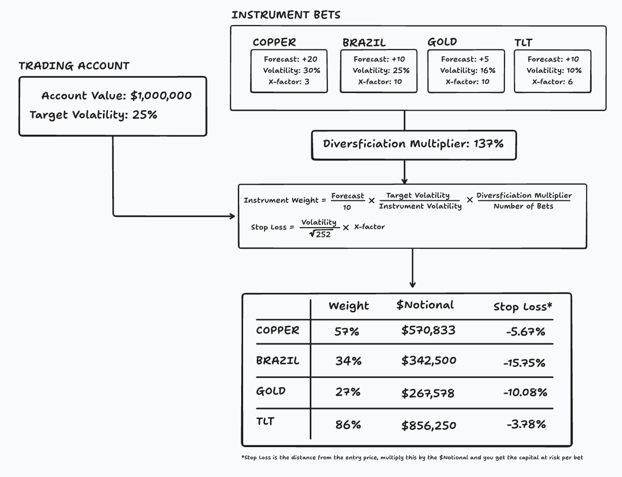
Jane is a global macro trader who draws on her experience in markets and macroeconomics to form views on various assets. She aims to capture major trends and ride them until exhaustion. She has consistently achieved a Sharpe ratio of 0.50 over the years and is managing an account value of $1mil. Based on our table mapping Sharpe Ratios to volatility targets, she chooses to run a 25% volatility target at the portfolio level.

Given the current macroeconomic environment, Jane believes copper is the next metal poised for a strong upward move. She is very bullish and assigns a forecast of +20. She also calculates the one-month realized volatility of copper at 30%.

Jane is also bullish on Brazilian equities, believing the bull run is just beginning. She assigns a forecast of +10 and measures a volatility of 25%.

She has been riding the gold trend for the past year, but now views the risk-reward as less attractive. She remains mildly bullish with a forecast of +5 and measures a volatility of 16%.

Finally, Jane is bullish on TLT, believing the bond market is overpricing strong US economic growth and underpricing the probability of a slowdown. She assigns a forecast of +10 and measures a volatility of 10%.

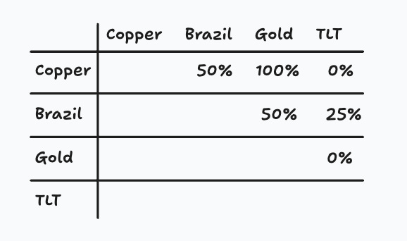
Using the recommended correlations by asset class, we can construct the following correlation matrix for Jane’s bets, yielding an average correlation of 37.5% ((50% + 100% + 0% + 50% + 25% + 0%) / 6).

To obtain the diversification multiplier, we reuse the expected volatility of the portfolio:

\(\begin{align*} V_p &= \frac{\sigma^2}{N} + \left(1 - \frac{1}{N}\right) \bar{\rho} \sigma^2 \\ &= \frac{0.20^2}{4} + \left(1 - \frac{1}{4}\right) \times 0.375 \times 0.20^2 \\ &= 0.02125 \end{align*}\)

and we get:

\(\begin{align*} \text{Diversification Multiplier} &= \frac{\text{Volatility Target}}{\sqrt{V_p}} \\ &= \frac{0.25}{\sqrt{0.02125}} \\ &= 1.37 \end{align*} \)

Now, Jane can apply the sizing algorithm to each bet:

A few observations:

• The total notional exposure is $2,037,161. The portfolio operates with 103.71% leverage (total net exposure is 203.71%), meaning Jane needs a margin account and will borrow shares or use futures.

• Copper receives a very large weight of 57% due to the +20 forecast and the 25% target volatility. Do not assign a +20 forecast lightly; it will significantly increase portfolio risk.

• Keep in mind that we are dealing with risk-adjusted bets. If an instrument’s volatility rises, you must recompute the weights. For example, if copper becomes more volatile, Jane will need to recalculate its instrument weight, which will reduce it, requiring her to sell some exposure.

Web App’s sizing tool

Now that you have a good understanding of how the system works, I can finally introduce the web app’s sizing tool, available here:

https://app.markethitchhiker.com/

You will find the sizing tool on the Trades page, nested within the Sizing Tool view.

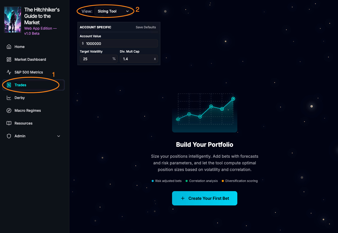
When creating a new bet, the app will prompt you to select the type of asset you would like to add:

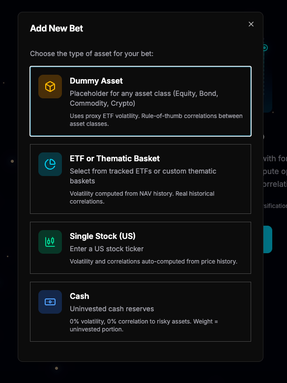
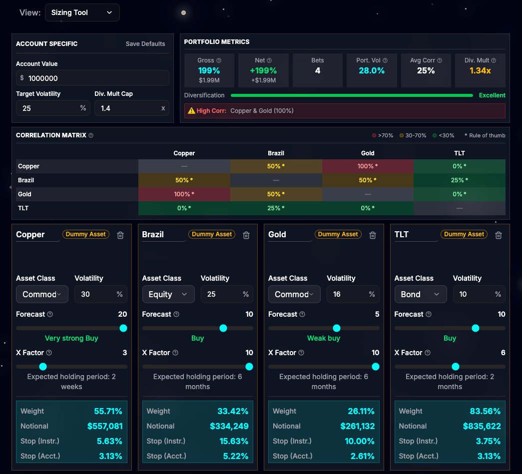
The Dummy Asset option allows you to add a bet on a theoretical asset, where you can manually set the asset class and volatility. By adding four dummy bets, we can recreate Jane’s portfolio as computed in the previous section:

If you prefer to create bets on real assets, you can use other bet types, such as “ETF or Thematic Basket” or “Single Stock” (any ticker quoted in the US). I have recreated Jane’s portfolio below using real ETFs:

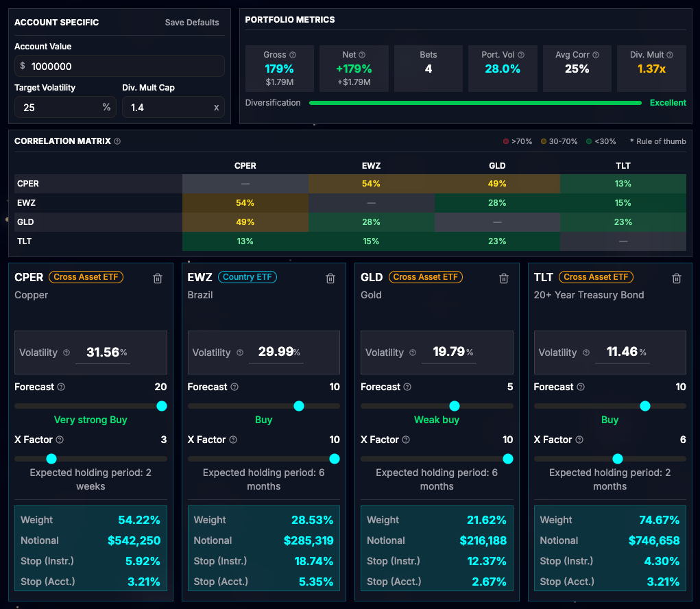
By using real assets, the app automatically calculates the actual volatility for each instrument with a conservative approach and computes the correlation matrix based on historical returns. The resulting weights differ slightly from those calculated with dummy assets, but they remain quite close. The portfolio metrics section also provides a handy overview of how well the portfolio is constructed.

The bets are saved automatically, so you do not need to recreate them the next time you log into the website.

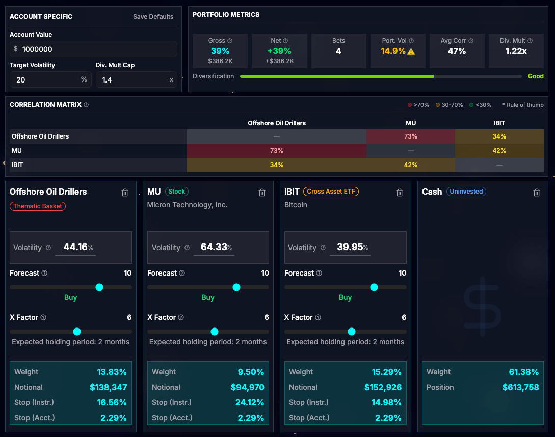
The final bet type you can add is “Cash,” which is actually a very useful option. Imagine you have three strong investment ideas for 2026:

• A thematic basket: long offshore oil drillers

• A single stock: long Micron (MU)

• An ETF: long IBIT

Like me, however, you prefer to run an average of four bets with a 20% target volatility. This provides concentration while still capturing diversification benefits. If you currently lack strong conviction for a fourth idea, using only three bets in the sizing tool would make the portfolio too aggressive. Adding a fourth bet of the Cash type solves this: the weights will be computed assuming four total bets. Indeed, when calculating the instrument weight for a given bet, we divide by the total number of bets:

\(\begin{align*} \text{Instrument Weight} &= \frac{\text{Forecast}}{10} \times \frac{\text{Target Volatility}}{\text{Instrument Volatility}} \\ &\times \frac{\text{Diversification Multiplier}}{\text{Number of Bets}} \end{align*} \)

Once you gain conviction in a new investment or trade idea, you can remove the cash bet and add the new one.

In a similar way, if you get stopped out on a trade but lack another idea, simply replace the stopped-out bet with a cash bet. This keeps the weights of the other bets unchanged. While you will undershoot your portfolio target volatility, you will avoid taking on overly concentrated risk.

Having Cash bets also provides a vital psychological benefit: it frames "doing nothing" as an active, risk-managed choice. It prevents you from forcing a mediocre trade just to fill the portfolio, allowing you to wait patiently for your next high-conviction setup.

Summary

This guide introduces a systematic framework for position sizing that rejects arbitrary rules like risking a flat 1% per trade. Instead, it positions capital at risk as an output of a deliberate system driven by three key inputs: your discretionary forecast, annual portfolio volatility target, and normalized stop-loss distance (the X-factor).

To apply this effectively, focus on these core principles:

• Forecasting and Conviction: Assign trades a score from -20 to +20, with +/-10 as the default for standard confidence. Beginners should limit to +/-10 until building a proven track record; reserve +/-20 for rare “Perfect Storm” alignments.

• Volatility Targeting: Assess your risk tolerance by mapping a conservative expected Sharpe Ratio to an annual volatility goal (e.g., 25% for SR 0.5), creating a psychological and financial buffer via half-Kelly sizing.

• X-Factor Alignment: Normalize stop-loss distance in daily standard deviations to match expected holding periods. A lower X-factor shortens trades and alters risk profiles, fostering positive skew.

• Diversification and Scaling: Use a diversification multiplier to counter “diworsification” (over-diversifying into correlated risks) or volatility undershoots. Aim for the sweet spot: 4-5 risk-adjusted bets with ~50% average correlation for balanced benefits.

• Practical Implementation: Leverage the Market Hitchhiker web app to automate calculations for real assets, thematic baskets, or dummy/cash placeholders, ensuring consistent risk even during idea droughts.

This approach compels you to address total annual risk upfront, delivering consistent volatility and sustainable performance. Though frequent stops can test your resolve (embracing uncertainty over illusory certainty), it’s the essential trade-off for averting deep drawdowns and letting winners thrive.

To apply this framework, consider subscribing to The Hitchhiker’s Guide to the Market. The free tier offers regular updates, while paid subscribers gain full access to the web app at https://app.markethitchhiker.com/, including tools for position sizing, thematic baskets, and other trading features. Paid members also get access to my open trades, which apply the Forecast and X-factor system described here, giving you the key inputs to size them intelligently in your own portfolio.

As an example, here’s a screenshot of some recently closed trades using this approach: